Decety et al., The Negative Association between Religiousness and Children’s Altruism across the World, Current Biology (2015), http://dx.doi.org/10.1016/j.cub.2015.09.056
Science proves that Daryl caused this page. (source)
How it looked in the headlines (5-8 Nov 2015)
Study Shows Non-Religious Kids Are More Altruistic and Generous Than Non-Religious Ones (TIME)
Religious children more punitive, less likely to display altruism (Boing Boing)
Study: Religious children less altruistic, more mean than nonreligious kids (Chicago Sun-Times)
Religious Kids Aren’t as Good at Sharing, Study Finds (Yahoo Parenting)
Study: Religion Makes Children Less Generous (Newser)
Religion doesn’t make kids more generous or altruistic, study finds (LA Times)
Religious children are meaner than their secular counterparts, study finds (The Guardian)
Being religious makes you less generous, study finds (metro.co.uk)
Kinder Without God: Kids Who Grow Up In A Religious Home Less Altruistic Than Those Without Religion (Medical Daily)
Surprise! Science proves kids with religious upbringings are less generous — and so are adults (rawstory.com, the Medical Daily story reposted with a new headline)
Well, that last one is a surprise – where did adults come into it?! Part of that story says:
It seems all these quotes are from a press release (“media alert”) from Cell Press, which refers to “new evidence reported in the Cell Press journal Current Biology on November 5”. It says the study was to “examine the influence of religion on the expression of altruism”, no mention of a hypothesis.
Decety’s words in the press release are exactly as quoted above. Which is very strange, unfortunately and carelessly worded, to the point of being misleading if not false. It sounds like the study shows something about adults. From my fairly brief look at the study so far, the only thing it shows about adults is that religious adults rate their children as having more “empathy and sensitivity for justice” than non-religious adults did, and more than they actually have.
There’s no by-line, but there’s a “Media Contact”: Joseph Caputo at cell.com – I guess he wrote that.
Possible problems/issues/questions that come to mind reading the paper
● they don’t mention in their paper that they were testing a hypothesis, if that’s what they were doing, although it gives that feeling. (That they believed their conclusion already, and were looking to gather evidence.) Is that..how these things should be done?!
● “caregivers also completed the Duke Religiousness Questionnaire (DRQ) [32], which assesses the frequency of religious attendance rated on a 1–6 scale from never to several times per week (frequency of service attendance and at other religious events), and questions regarding the spirituality of the household (1–5 scale; see DRQ). Average religious frequency and religious spirituality composites were created, standardized, and combined for an average overall religiousness composite.”
So it’s How often you go to church/mosque? uh… The most religious ppl ive known were not those who went to church a lot. negative correlation, maybe.
● “Maternal Education : As a metric for socioeconomic status, parents were asked to specify the level of education of the mother.” hehe! They give correlations to 3 decimal places with socio-economic status. And it’s based on – THIS?! (it seems, a 1-6 scale) (and <1% were '1' - 0-5 years of education)
● the Altruism score (what the paper is all about) is scored 1-10, based on how many stickers out of 10 the child gave away (to an unknown child who didn't get any). Imagine giving all 10 away. To me, this would suggests they don't care for stickers, more than that they're altruistic. If someone gave away ALL their lunch, it would suggest they're not hungry.
● the average ages differed in different countries, from ave. of 7.5 to 9
● different groups (diff. countries) mixed together. Maybe there are very different correlations in different countries. Or would they have mentioned it, if there were?
● was it double blind? It doesnt say. (Maybe it's considered obvious) Did the assistants doing the stickers test know anything about the children? Maybe some of them had visible religious markers, clothing etc?
● the graph presented seems like a big jumble. Why is a linear regression (a plane through the 3D graph) used? It seems likely in such things that the pattern, if there is one, would be a curve of some kind.
● did they make predictions? Or was it a fishing expedition? not clear. "To examine the influence of religion on the expression of altruism, ..."
● correlations with country. these are of a different nature than data with a scale.
Firstly, some basics of:
research methods
I. Measuring two variables for each individual: The correlational method
+++++One method for examining the relationship between variables is to simply measure the two variables for each individual. For example, research has demonstrated a relationship between sleep habits and academic performance for college students. The researchers used a survey to measure wake-up time and school records to measure academic performance for each student.
+++++The researchers then look for consistent patterns in the data to provide evidence for a relationship between variables. For example, as wake-up time changes from one student to another, is there also a tendency for academic performance to change?
Limitations: The results from a correlational study can demonstrate the existence of a relationship between two variables, but they do not provide an explanation for the relationship. In particular, a correlational study cannot demonstrate a cause-and-effect relationship.
II. Comparing two (or more) groups of scores: Experimental and nonexperimental methods
+++++The second method for examining the relationship between two variables involves the comparison of two or more groups of scores. In this situation, the relationship between variables is examined by using one of the variables to define the groups, and then measuring the second variable to obtain scores for each group.
+++++A. The Experimental Method.
+++++The goal of an experimental study is to demonstrate a cause-and-effect relationship between two variables, by trying to show that changing the value of one variable causes changes to occur in the second variable. The experimental method has two unique characteristics:
+++++1. Manipulation. The researcher manipulates one variable by changing its value from one level to another. A second variable is observed (measured) to determine whether the manipulation causes changes to occur.
+++++2. Control. The researcher must exercise control over the research situation to ensure that other, extraneous variables do not influence the relationship being examined.
+++++There are two general categories of variables that researchers must consider:
+++++1. Participant Variables. These are characteristics such as age, gender, and intelligence that vary from one individual to another.
+++++2. Environmental Variables. These are characteristics of the environment such as lighting, time of day, and weather conditions.
+++++Researchers typically use three basic techniques to control other variables. First, the researcher could use random assignment, which means that each participant has an equal chance of being assigned to each of the treatment conditions. The goal of random assignment is to distribute the participant characteristics evenly between the two groups so that neither group is noticeably smarter (or older, or faster) than the other. Random assignment can also be used to control environmental variables. For example, participants could be assigned randomly for testing either in the morning or in the afternoon. Second, the researcher can use matching to ensure equivalent groups or equivalent environments. For example, the researcher could match groups by ensuring that every group has exactly 60% females and 40% males. Finally, the researcher can control variables by holding them constant. For example, if an experiment uses only 10-year-old children as participants (holding age constant), then the researcher can be certain that one group is not noticeably older than another.
+++++In the experimental method, one variable is manipulated while another variable is observed and measured. To establish a cause-and-effect relationship between the two variables, an experiment attempts to control all other variables to prevent them from influencing the results.
+++++An experimental study evaluates the relationship between two variables by manipulating one variable (the independent variable) and measuring one variable (the dependent variable). In an experiment only one variable is actually measured. This is different from a correlational study, in which both variables are measured and the data consist of two separate scores for each individual.
+++++Whenever a research study allows more than one explanation for the results, the study is said to be confounded because it is impossible to reach an unambiguous conclusion.
Control Groups in an Experiment. Often an experiment will include a control group in which the participants do not receive any treatment. The scores from these individuals are then compared with scores from participants who do receive the treatment, the experimental group. The goal is to demonstrate that the treatment has an effect by showing that the scores in the treatment group are substantially different from the scores in the control group.
+++++B. Nonexperimental methods: nonequivalent groups and pre-post studies
+++++In informal conversation, there is a tendency for people to use the term experiment to refer to any kind of research study. However, that the term only applies to studies that satisfy the specific requirements outlined earlier. In particular, a real experiment must include manipulation of an independent variable and rigorous control of other, extraneous variables. As a result, there are a number of other research designs that compare groups of scores but are not true experiments. This type of research study is classified as nonexperimental.
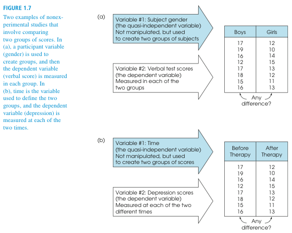
+++++The top part of Figure 1.7 shows an example of a nonequivalent groups study comparing boys and girls. Notice that this study involves comparing two groups of scores (like an experiment). However, the researcher has no ability to control the assignment of participants to groups — the males automatically go in the boy group and the females go in the girl group. Because this type of research compares preexisting groups, the researcher cannot control the assignment of participants to groups and cannot ensure equivalent groups. Other examples of nonequivalent group studies include comparing 8-year-old children and 10-year-old children or comparing people with an eating disorder and those with no disorder. Because it is impossible to use techniques like random assignment to control participant variables and ensure equivalent groups, this type of research is not a true experiment.
+++++The bottom part of Figure 1.7 shows an example of a pre–post study comparing depression scores before therapy and after therapy. The two groups of scores are obtained by measuring the same variable (depression) twice for each participant; once before therapy and again after therapy. In a pre–post study, however, the researcher has no control over the passage of time. The “before” scores are always measured earlier than the “after” scores. Although a difference between the two groups of scores may be caused by the treatment, it is always possible that the scores simply change as time goes by. For example, the depression scores may decrease over time in the same way that the symptoms of a cold disappear over time. In a pre–post study, the researcher also has no control over other variables that change with time. For example, the weather could change from dark and gloomy before therapy to bright and sunny after therapy. In this case, the depression scores could improve because of the weather and not because of the therapy. Because the researcher cannot control the passage of time or other variables related to time, this study is not a true experiment.
Terminology in nonexperimental research Although the two research studies shown in Figure 1.7 are not true experiments, they produce the same kind of data that are found in an experiment. In each case, one variable is used to create groups, and a second variable is measured to obtain scores within each group. In an experiment, the groups are created by manipulation of the independent variable, and the participants’ scores are the dependent variable. The same terminology is often used to identify the two variables in nonexperimental studies. That is, the variable that is used to create groups is the independent variable and the scores are the dependent variable. For example, the top part of Figure 1.7, gender (boy/girl), is the independent variable and the verbal test scores are the dependent variable. However, you should realize that gender (boy/girl) is not a true independent variable because it is not manipulated. For this reason, the “independent variable” in a nonexperimental study is often called a quasi-independent variable. -ESBS
variables
constructs and operational definitions
+++++Some variables, such as height, weight, and eye color are well-defined, concrete entities that can be observed and measured directly. On the other hand, many variables studied by behavioral scientists are internal characteristics that cannot be observed or measured directly. However, we all assume that these variables exist and we use them to help describe and explain behavior. For example, we say that a student does well in school because he or she is intelligent. Or we say that someone is anxious in social situations, or that someone seems to be hungry. Variables like intelligence, anxiety, and hunger are called constructs, and because they are intangible and cannot be directly observed, they are often called hypothetical constructs.
+++++Although constructs such as intelligence are internal characteristics that cannot be directly observed, it is possible to observe and measure behaviors that are representative of the construct. For example, we cannot “see” intelligence but we can see examples of intelligent behavior. The external behaviors can then be used to create an operational definition for the construct. An operational definition measures and defines a construct in terms of external behaviors. For example, we can measure performance on an IQ test and then use the test scores as a definition of intelligence. Or hunger can be measured and defined by the number of hours since last eating.
types of variables and scales
+++++A discrete variable consists of separate, indivisible categories. No values can exist between two neighboring categories. e.g. integers, male/female, occupation.
+++++For a continuous variable, there are an infinite number of possible values that fall between any two observed values. A continuous variable is divisible into an infinite number of fractional parts.
+++++A nominal scale consists of a set of categories that have different names. Measurements on a nominal scale label and categorize observations, but do not make any quantitative distinctions between observations.
+++++An ordinal scale consists of a set of categories that are organized in an ordered sequence. Measurements on an ordinal scale rank observations in terms of size or magnitude.
+++++An interval scale consists of ordered categories that are all intervals of exactly the same size. Equal differences between numbers on the scale reflect equal differences in magnitude. However, the zero point on an interval scale is arbitrary and does not indicate a zero amount of the variable being measured.
+++++A ratio scale is an interval scale with the additional feature of an absolute zero point. With a ratio scale, ratios of numbers do reflect ratios of magnitude. – ESBS
Well, to read the paper and understand it at all I’ll have to learn some :
Basic Statistics
 , univariate analysis of variance, visual Likert scale, Duke Religiousness Questionnaire etc.
The 3 averages
+++++The mean is what’s usually called the average in everyday life – the total of all scores, divided by the number of scores (sample size). It’s different from the median (1/2 the scores are higher, 1/2 lower) and the mode, the most common value. The mode may not exist, e.g. if all the values are different, or there may be 2 or more modes.
variable, sample, statistic, population, parameter
A sample is a set of individuals selected from a population, usually intended to represent the population in a research study.
A variable is a characteristic or condition that changes or has different values for different individuals.
To demonstrate changes in variables, it is necessary to make measurements of the variables being examined. The measurement obtained for each individual is called a datum or, more commonly, a score or raw score. The complete set of scores is called the data set, or simply the data.
When describing data, it is necessary to distinguish whether the data come from a population or a sample. A characteristic that describes a population — for example, the average score for the population — is called a parameter. A characteristic that describes a sample is called a statistic. – ESBS
A statistic is a value, usually a numerical value, that describes a sample. A statistic is usually derived from measurements of the individuals in the sample. ”
Q. How is it possible to measure individuals “in the population”? Isn’t the existence of statistics due to the difficulty that populations are often too big to study each individual, and a sample must be studied??
variance and standard deviation
OK, say you have a lot of test scores. You can find the average, but that won’t tell you whether everyone got that score, or the scores varied wildly. This is what variance and standard deviation are for – to describe how close around the average the scores are – the distribution.
The sample variance = average squared deviation from the average score. Subtract the average from every score, square these deviations and find their average, i.e. add them together and divide by the number of samples. 
The standard deviation is the square root of this.
e.g. if the data is 2, 4, 6, then the average is  , the variance is
  and
and  .
.
 ,
,  , and
, and  . and come from the words standard deviation squared. MS comes from the words mean square. When variance is calculated from a population, it typically has just one symbol,
  (pronounced “sigma squared”), and is a parameter. (Remember, Latin letters are used for statistics, which are calculated from samples, and Greek letters are used with parameters, which are calculated from or hypothesized for populations.) – SBS
More commonly used in scientific papers and statistics software is:
unbiased variance =  , not
, not  , i.e.
and the standard deviation based on the unbiased variance, i.e.  . (In this example, all (both) the deviations are
  , so the
  should be 2!)
 instead of
  in the formula for the sample variance and sample standard deviation, where is the number of observations in a sample. This corrects the bias in the estimation of the population variance, and some (but not all) of the bias in the estimation of the population standard deviation, but often increases the mean squared error in these estimations. …This correction is so common that the term “sample variance” and “sample standard deviation” are frequently used to mean the corrected estimators (unbiased sample variation, less biased sample standard deviation), using . However caution is needed: some calculators and software packages may provide for both or only the more unusual formulation. – wikipedia
z scores, standardization and z distribution
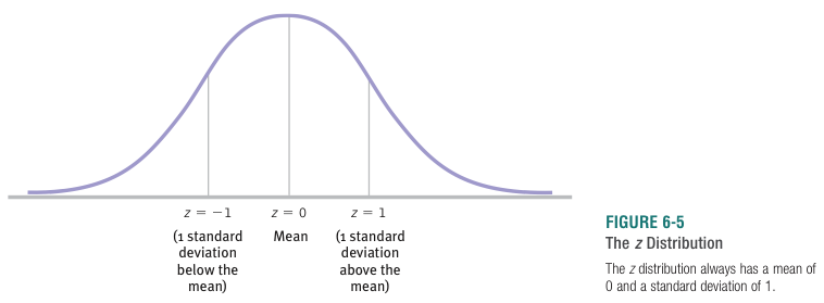
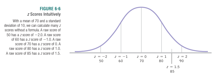
A  score is the difference of a particular score from the average, measured in units of standard deviations.
  scores make meaningful comparisons possible, by putting different variables on a common scale. The only information needed to convert a raw score to a score is the average and standard deviation of the population of interest.
![\[z\text{ score }= \frac{\text{individual score } - \text{population mean}}{\text{population standard deviation}}} = \frac{X-\mu}{\sigma}\]](https://www.adamponting.com/wp-content/ql-cache/quicklatex.com-604bc23a368ffef04d0fecb53f308070_l3.png "Rendered by QuickLaTeX.com")
To standardize is to convert all scores into scores.
correlation and covariance
Covariance is a shared corresponding variation between a pair of variables
r is Pearson’s correlation coefficient. It ranges from  (indicating perfect negative linear correlation) to
  (perfect positive linear correlation).
 = the average product of scores for the two variables.
● measures linear relationships only. (straight lines on the scatterplot)
● a few extreme scores – outliers – can influence greatly.
● it doesn’t specify a direction of influence
● mixing different groups can skew/hide correlations.
 (squared correlation coefficient) = the coefficient of determination, the proportion of variance shared by the 2 variables, the fraction of the variation in one variable that is explained by the other variable. It ranges between
  and .
and .
. That is the position that I think is the better one, but, as you will see when we come to the analysis of variance, I am not always consistent myself. For a more extensive discussion of this issue, see Grissom and Kim (2012, p. 140). – FSBS p243
Correlation, even strong correlation, does not imply causation!
= .62linear regression
linear regression,  standardized regression coefficient
“stickers shared as the dependent variable and age (1-year bins) …( = 0.410, p < 0.001)" - This means, graphing age (X axis, 5-12) against stickers shared (Y axis, 0-10), and working out the slope of the line that minimizes the sum of squared distances between it and the data points - after first converting the data to standardized scores. (a mean of 0 and standard deviation (SD?) of 1). Then the slope would be equal to the standardized regression coefficient (), not the ‘raw’ coefficient for nonstandardized data
  . When there’s one predictor variable – here age, is the same as the correlation coefficient.
adjusted = 0.194).”; I don’t yet know what that means.
Why do we need both regression AND correlation?
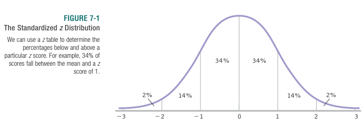
t distribution and t tests
 distribution
distribution instead of a distribution when sampling requires us to estimate the population standard deviation from the sample standard deviation, [and] when we don’t know the population standard deviation or when we compare two samples to each other. …There are many distributions — one for each possible sample size. As the sample size gets smaller, we become less certain about what the population distribution really looks like, and the distributions become flatter and more spread out. However, as the sample size gets larger, the distributions begin to merge with the distribution because we gain confidence as more and more participants are added to our study.
Estimating Population Standard Deviation from a Sample
+++++Before we can conduct a single-sample test, we have to estimate the standard deviation. To do this, we use the standard deviation of the sample data to estimate the standard deviation of the entire population. Estimating the standard deviation is the only practical difference between conducting a test with the distribution and conducting a test with a distribution. Here is the standard deviation formula that we have used up until now with a sample: 
+++++We need to make a correction to this formula to account for the fact that there is likely to be some level of error when we’re estimating the population standard deviation from a sample. Specifically, any given sample is likely to have somewhat less spread than does the entire population. One tiny alteration of this formula leads to the slightly larger standard deviation of the population that we estimate from the standard deviation of the sample. Instead of dividing by  , we divide by
  .
.
single-sample test – A hypothesis test in which we compare data from one sample to a population for which we know the mean but not the standard deviation.
independent-samples test – A hypothesis test used to compare two means for a between-groups design, a situation in which each participant is assigned to only one condition.
GLOSSARY (things I haven’t read/written about yet)
bivariate – linked to 2 variables.
ANOVA (analysis of variance) – A hypothesis test typically used with one or more nominal independent variables (with at least three groups overall) and a scale dependent variable.
ANCOVA (analysis of covariance) – A type of ANOVA in which a covariate is included so that statistical findings reflect effects after a scale variable has been statistically removed.
covariate – A scale variable that we suspect associates, or covaries, with the independent variable of interest.
Bonferroni test – A post-hoc test that provides a more strict critical value for every comparison of means; sometimes called the Dunn Multiple Comparison test.
post-hoc test – A statistical procedure frequently carried out after we reject the null hypothesis in an analysis of variance; it allows us to make multiple comparisons among several means; often referred to as a follow-up test.
dependent variable – The outcome variable that we hypothesize to be related to, or caused by, changes in the independent variable.
independent variable – A variable that we either manipulate or observe to determine its effects on the dependent variable.
scale variable –
convenience sample – A subset of a population whose members are chosen strictly because they are readily available, as opposed to randomly selecting participants from the entire population of interest.
[late 2015]
Update 2017
Nonreligious children aren’t more generous after all.
“A study finding that children with a Christian or Muslim upbringing were less altruistic than their non-religious counterparts made waves in 2015. However, new analysis of the data reveals that this is not actually the case. In the study, developmental psychologists looked at five- to twelve-year-olds in Canada, China, Jordan, Turkey, South Africa, and the United States. The children were given stickers and provided the opportunity to share them with peers who were not present. The number of stickers shared provided a quantifiable indicator of each child’s altruism.
After interpreting the resulting data, the study’s authors concluded that children from religious families were less generous. However, new analysis shows that the original study failed to adequately control for the children’s nationality. After correcting this error, the authors of a newly published paper found no relationship between religiosity and generosity.”
bibliography/references
ESBS = Gravetter and Wallnau – Essentials of Statistics for the Behavioral Sciences, 8th Ed. (2014)
FSBS = D.C. Howell – Fundamental Statistics for the Behavioral Sciences
SBS = Nolan, Heinzen – Statistics for the Behavioral Sciences (2010)