These images were made by mucking around with equations producing (to quote from the Pickover chapter that inspired them) “time-discrete phase planes associated with the cyclic systems:
(1) 
In phase space each dimension can represent one of the variables in the differential equation. …Here, these functions are generally of the form often found in frequency modulation synthesis applications:
![\[f(x)=\sin[x+\sin(\rho x)]\]](https://www.adamponting.com/wp-content/ql-cache/quicklatex.com-888ac8f2d70864f0029a7b6ff9154080_l3.png "Rendered by QuickLaTeX.com")
By modulating a sine wave (often called the “carrier”) by another with a different frequency (controlled by  ), a large variety of complex waveforms can be generated … Using this technique, a graphically “rich” function can be produced with only a small number of input parameters.
The discretization of Equation  for implementation on a computer takes the following simple form (known as the forward Euler approximation):
![\[ \left\{ \begin{array}{lr} x_{t+1}-x_t=-hf(y_t)\\ y_{t+1}-y_t=hf(x_t) \end{array} \right. \]](https://www.adamponting.com/wp-content/ql-cache/quicklatex.com-95e44bf2d41790e0ec89f8c79a9ba53b_l3.png "Rendered by QuickLaTeX.com")
where  is a constant known as the step size of the numerical solution. In this section,
  is kept small (
 ). … Despite the phase portraits’ complexity, they possess universal features shared by entire classes of nonlinear processes. For example, a range of real physical systems can be described by similar systems of differential equations.”
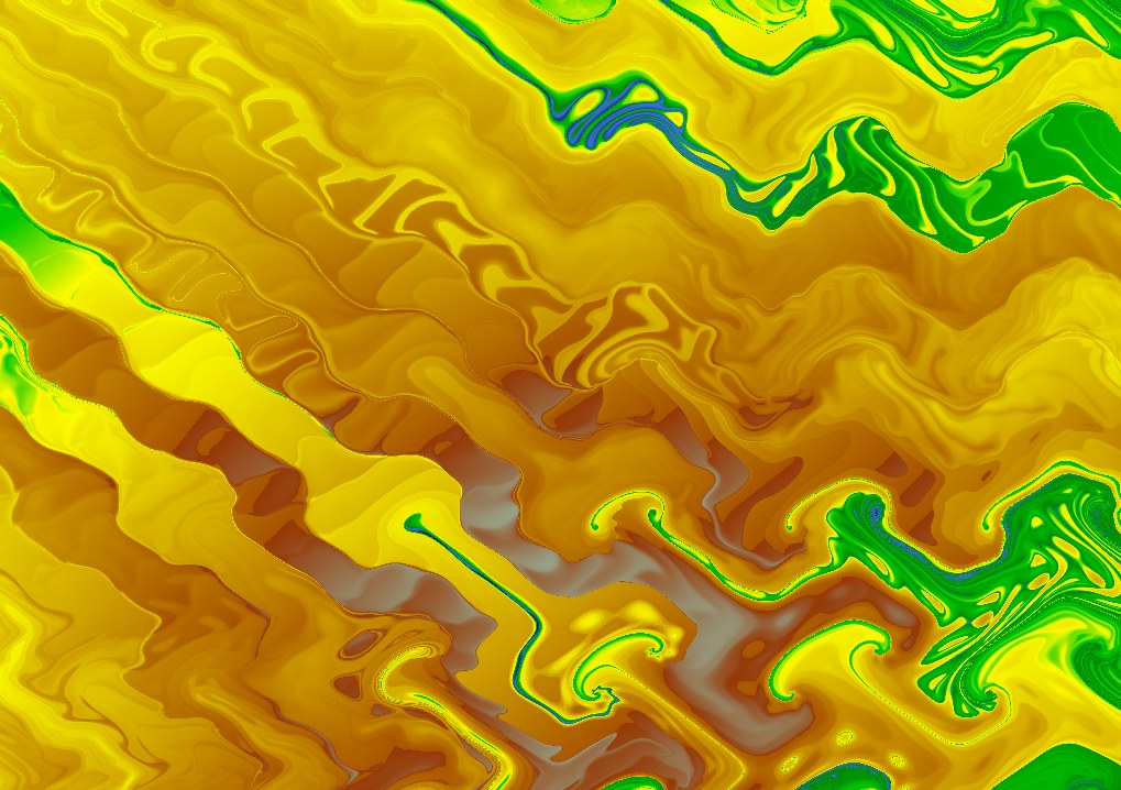
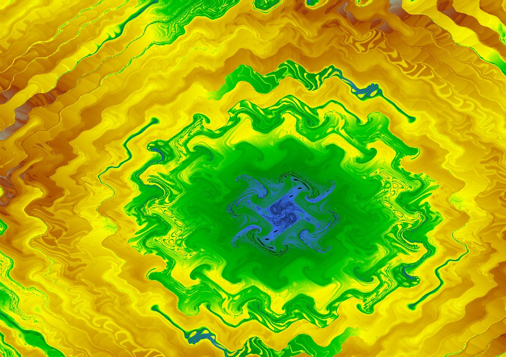
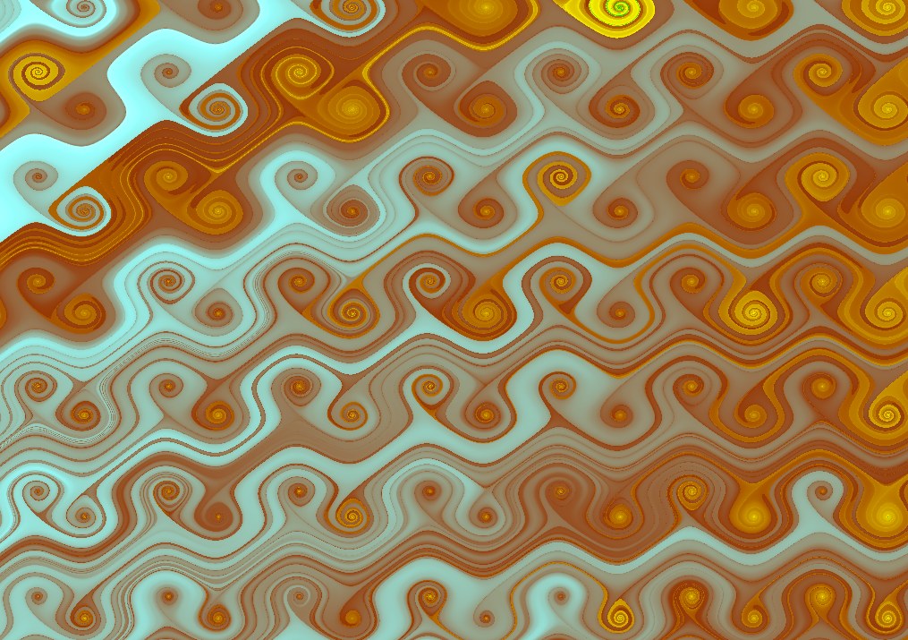
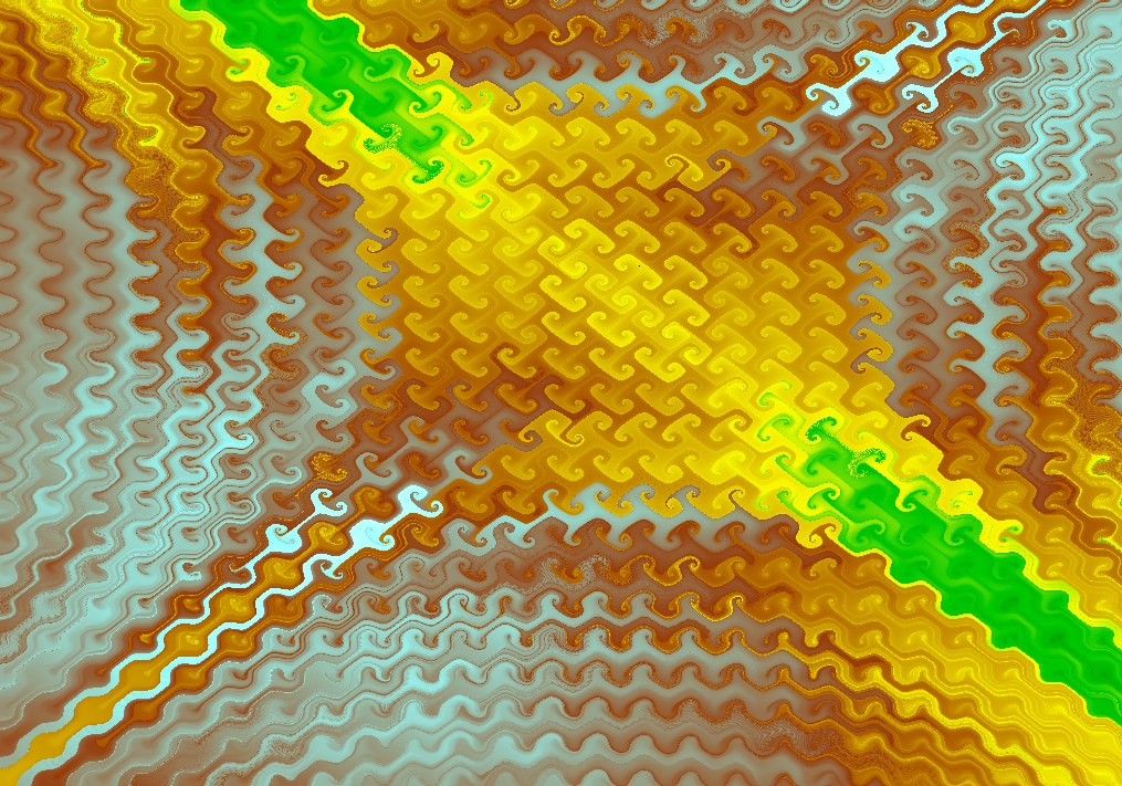
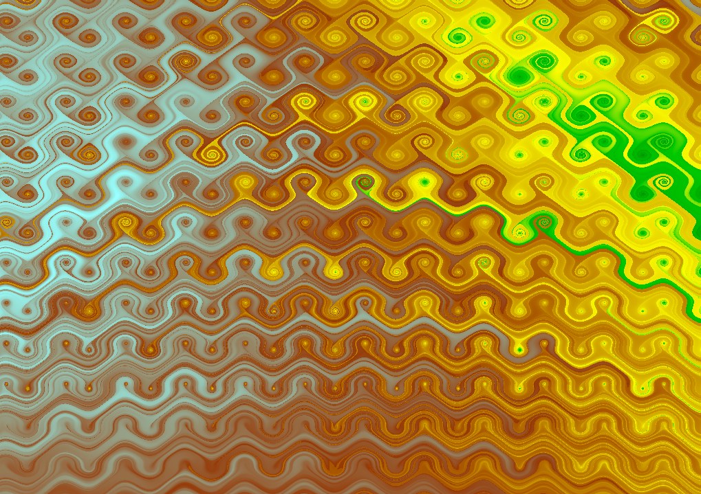
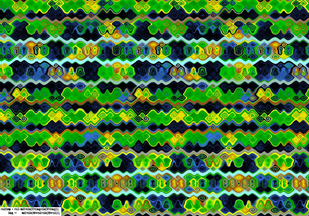
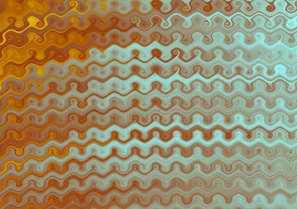
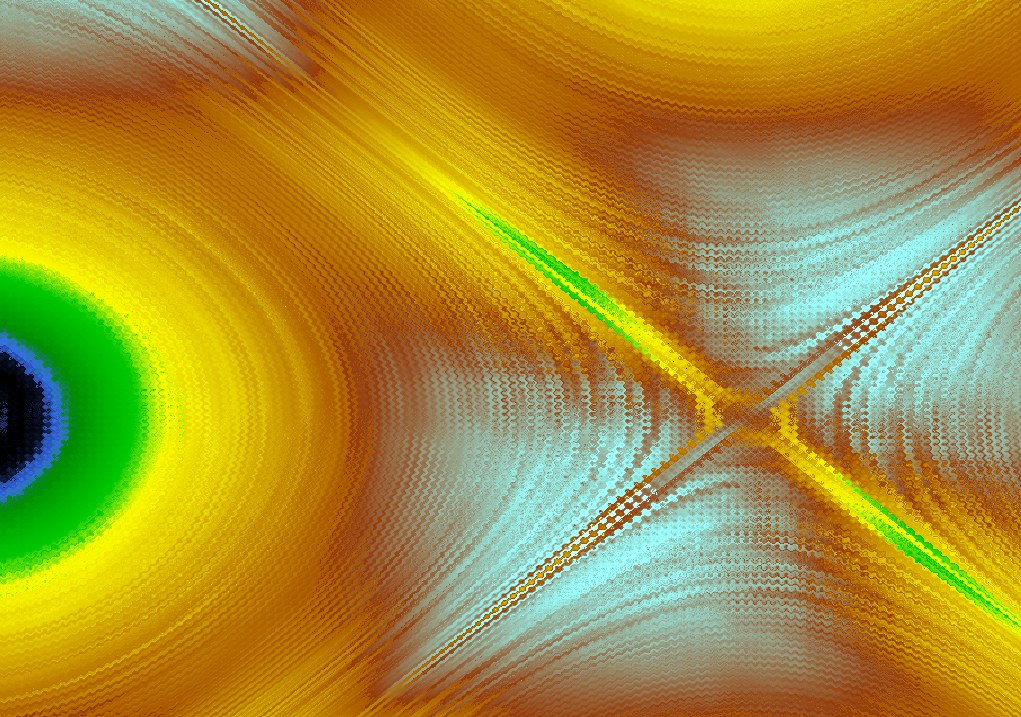
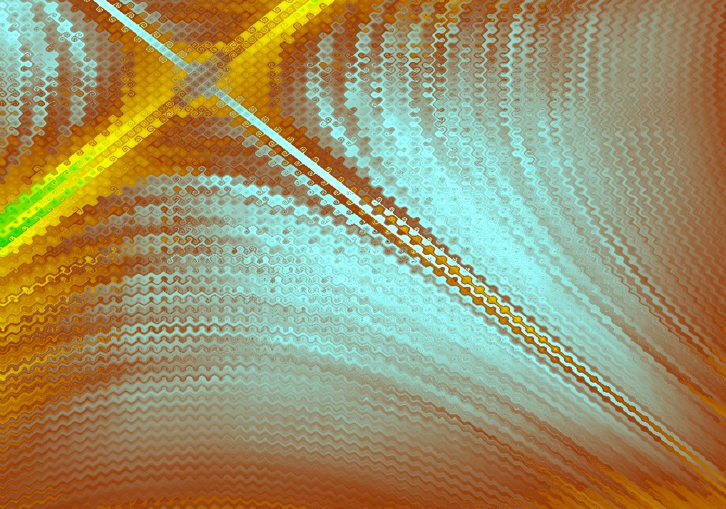
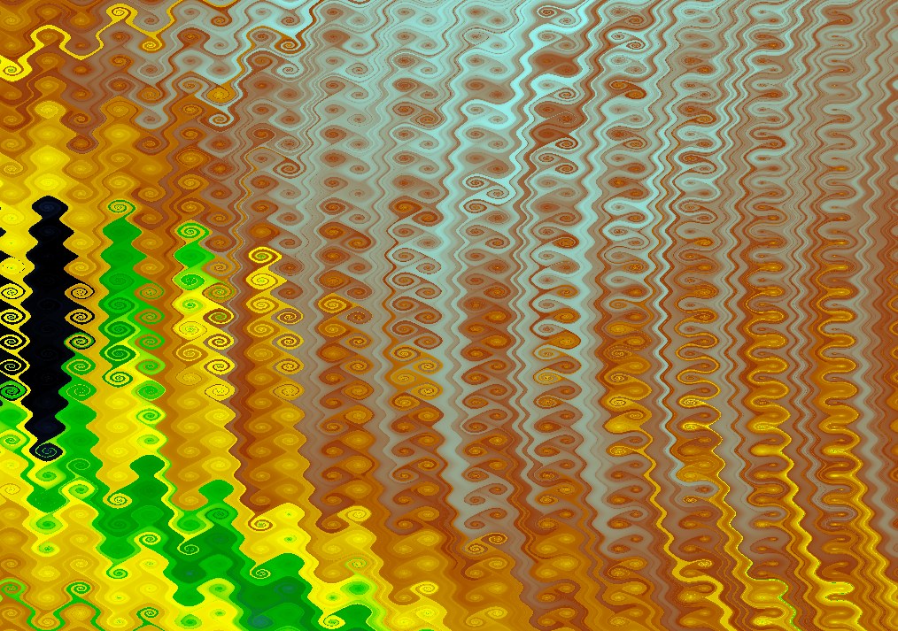
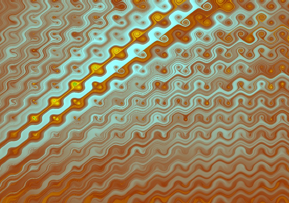
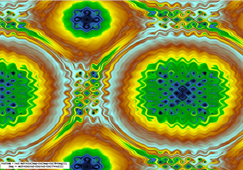
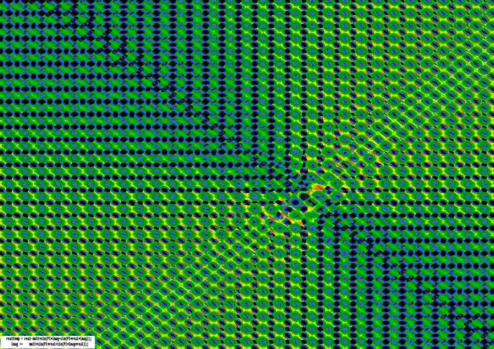
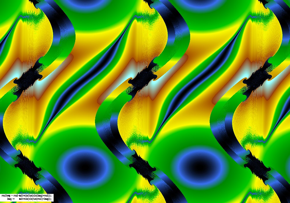
I’ve not used the trajectories of randomly-chosen points, as he does, but instead traced the trajectory of every point on the screen a certain small number of steps, and colouring them according to the distance travelled from the starting point, with colours similar to those used in coloured relief maps – blue(ocean)  dark green light green yellow brown white(snow).
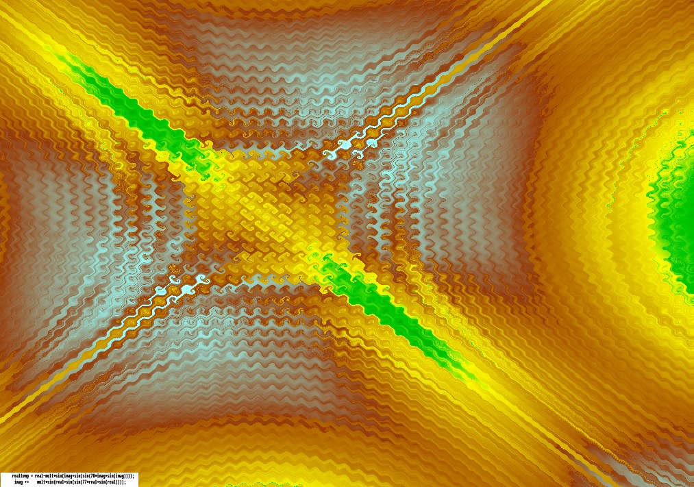
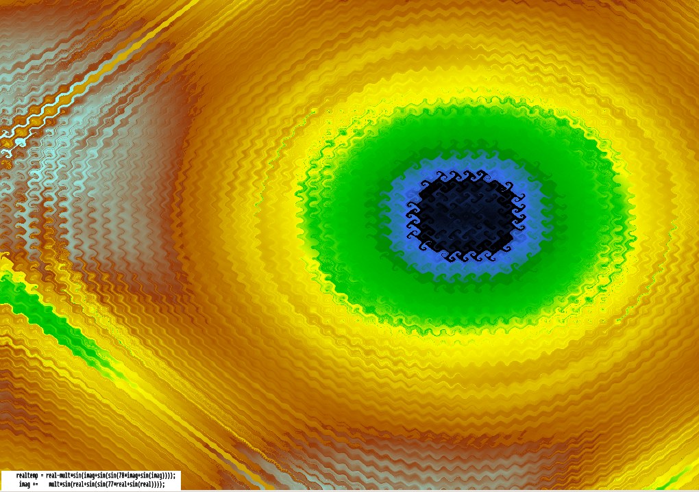
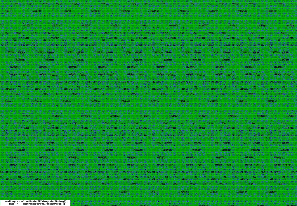
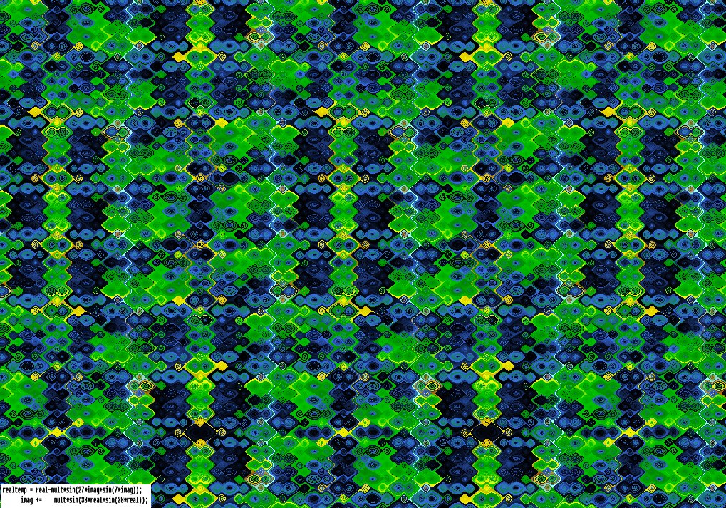
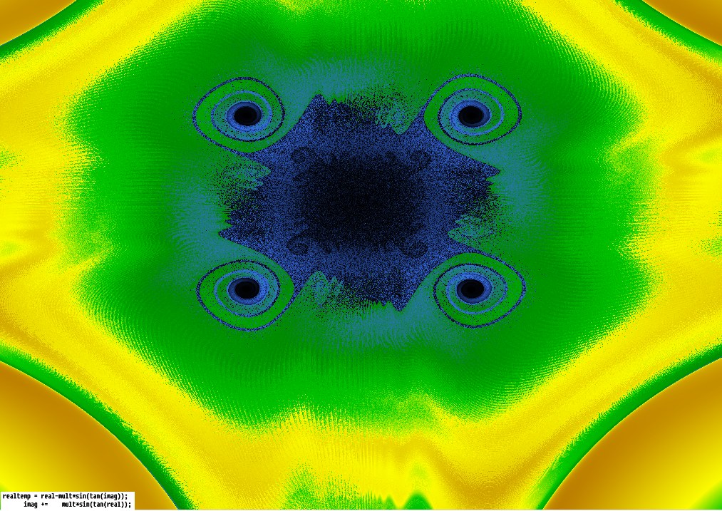
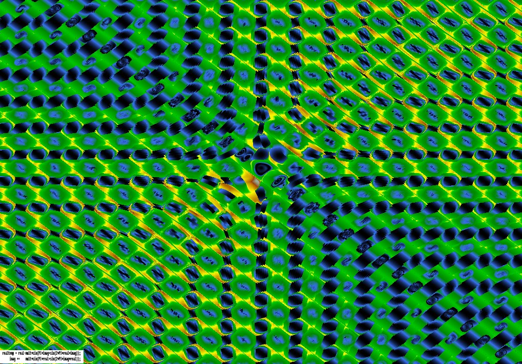
Some of the images have the 2 main equation lines pasted on them, from the program that drew them – e.g. the 11th picture below, the first one with a formula on it, says in C++ :
realtemp = real-mult*sin(27*imag+sin(7*imag));
imag += mult*sin(30*real+sin(28*real));
I made those numbers up pretty much randomly, to see what would happen. This translates into the above style as:
![\[\left\{\begin{array}{lr} x_{t+1}=x_t-h\sin(27y_t+\sin(7y_t))\\ y_{t+1}=y_t+h\sin(30x_t+\sin(28x_t)) \end{array} \right. \]](https://www.adamponting.com/wp-content/ql-cache/quicklatex.com-022b9726b85614dd87fcea512941291b_l3.png "Rendered by QuickLaTeX.com")
Computers, Pattern, Chaos and Beauty: Graphics from an Unseen World – Clifford Pickover, 1990